De-noising CMap L1000 Data

The Connectivity Map (CMap) is a conceptual, comprehensive linking of cellular signatures to genomic (i.e. mutation) and pharmacological (i.e. drug-mediated) effects. The CMap dataset is based on the L1000 assay (developed by the Broad Institute), which measures the mRNA abundance of 978 landmark genes plus 80 control genes from human cells.As with any assay, L1000 data is noisy. Experimental replicates (the same compound tested on the same cell line under the same conditions) often result in different levels of expression being measured. The experimental protocol attempts to accommodate some of this noise through five levels of preprocessing, but there is inevitably still some variance in the experimental replicate results in the final Level 5 dataset.Typically we want to determine a representative L1000 profile for a given compound, indicating its effect on transcriptional response. Compounds are assayed at different concentrations, as too low a dose may lead to no response, while too high a dose may produce toxic effects. Ideally, we want to find the lowest dose at which a compound exerts a significant signal. But it can be hard to find this concentration due to the noise.Below we show a dose-response plot for a subset of the CMap compounds, where “response” here means the median number of significantly modulated genes (p-value of 99%, i.e. a z-score greater than 2.575829 or less than -2.575829) in all Level 5 profiles for an experimental replicate (same cell line, time, dose concentration, and compound). Each line represents a single compound, where the colours are arbitrary.

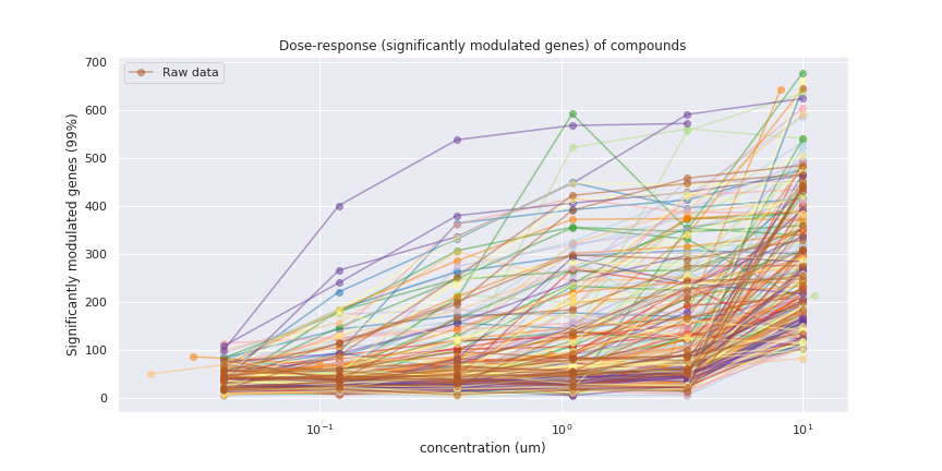It looks like all compounds show some activity at all concentrations. In a typical dose-response plot we would expect to see a threshold concentration at which activity starts, but the noise obscures the thresholds here.

Modelling the noise

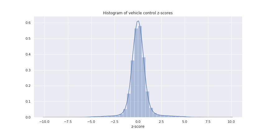
The CMap dataset contains 6467 vehicle control samples, meaning that the cell line was tested with no active compound (only the dimethyl sulfoxide vehicle). Theoretically these controls should show no response, so any modulation in the expression z-scores must be due to noise.We can visualize this noise by calculating the kernel density estimate of the control z-scores (below). Helpfully, it looks nice and simple: approximately Gaussian with mean 0 and standard deviation 1.

With this understanding of the noise, we can model it formally and try to remove it from the dataset.

Gaussian Mixture Models (GMMs)

Gaussian Mixture Models (GMMs) decompose a dataset into multiple Gaussian distributions. The user chooses how many Gaussians (components) are expected, and the Expectation Maximization (EM) algorithm finds the parameters of those components that best fit the data.We chose two components: one for the noise and one for the “signal” (real expression modulations in the L1000 assay). The noise was confirmed to be relatively Gaussian in the controls, so a GMM should find its parameters easily. The signal is less likely to be Gaussian because certain genes modulate together, but we can take advantage of the Central Limit Theorem and assume that the combination of all true gene modulations will look more Gaussian than any individual L1000 response.We can also set some constraints on the expected parameters of the Gaussian components. Each Gaussian component has 978 dimensions: one for each of the L1000 genes. Since we are using z-scores, we expect the mean of the noise component to be 0 and the variance to be 1 in all dimensions. Hence, the covariance matrix should be spherical. This constraint allows the GMM to more closely approximate the noise component, and therefore to discriminate better between signal and noise.

Results

After training the GMM on the L1000 data, we can use it as a classifier to separate “signal” Level 5 profiles from noise. The plot below shows the number of significantly modulated genes for three groups of L1000 profiles:

• The vehicle controls (in blue)
• The L1000 profiles classified as being noise (in orange)
• The L1000 profiles classified as being true expression modulation results (in green).

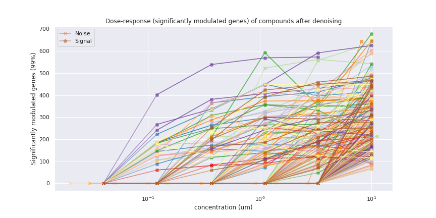
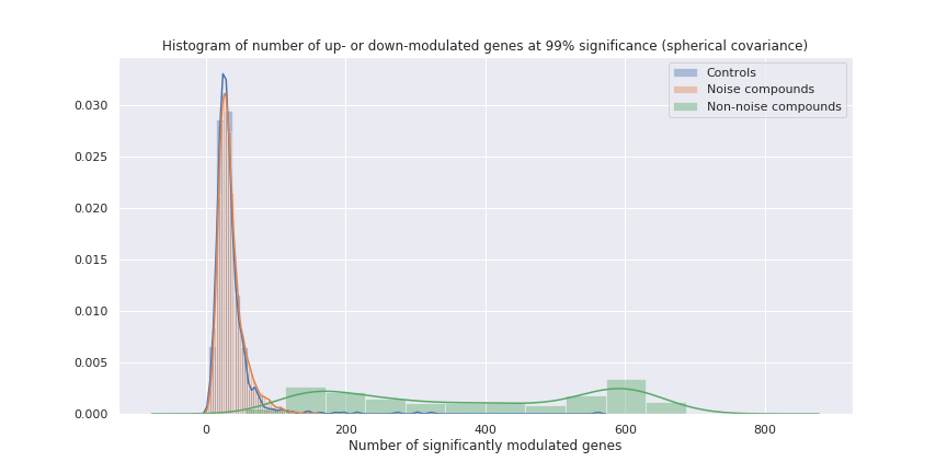The orange overlays the blue very closely, indicating that the GMM has modelled the noise accurately. As a result, we can be confident that the remaining profiles truly reflect expression modulations.With this knowledge, we can now redraw the dose-response plot from above with the noise points set to zero. This time it’s much easier to determine the threshold concentration for each compound, above which it starts to become active. We can also more clearly see the true activity of compounds which modulate fewer than 100 genes, which were previously just lost in the noise.

Conclusion

De-noising the L1000 data makes it easier to see true assay response, and pick a representative concentration for each compound.